QuickSort Algorithm

Here you’ll learn how to write a program for quicksort algorithm understand its theory, and using an example learn how its implemented.

Contrary to the name, this isn’t the fastest sorting algorithm out there, this will be clearer once the time complexity of QuickSort is discussed later. But first, let’s start with the algorithm approach.

What is the approach to QuickSort?

The objective is to have the given numbers in increasing order, the method we approach here is inherently simple, instead of juggling through all the elements at once what if we placed one element at its correct position at a time? To help to understand this, imagine the queue in the morning assembly of School, if you remembered your position say 5th from the front, it didn’t matter where others stood, you would be able to stand at your correct place and since everyone does the same, the students assemble in large numbers without creating stampede every morning.

Understanding Pivot

Here take a look at the following array, is this array sorted? No, but there is something particular about no 10, if you observe, the numbers less than 10 are on the left and the numbers greater than 10 are on the right, no matter if they aren’t sorted within themselves, we can be assured that 10 will be in this position when the array is sorted. This number with which we compare all the left and right side numbers is referred as a pivot.

So extended this same logic, imagine we change the pivot for the whole array then, in essence, we have solved the problem because pivot stays in its place after sorting, and since all have been pivoted we can surely conclude that we have completed the objective of creating a sorted array.
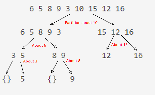
The process is not linear but follows a binary tree structure. In the above code the pivot 10 partitions the array into two smaller arrays of size 3 and 4 respectively, so we operate the same partition/pivot algorithm on those smaller arrays to create 4 new arrays so on and so forth.
Now let’s take a look at the program for the quicksort algorithm first and then the example will make the execution of the same much clearer.

Program for Quick Sort Algorithm

int partition(int *A,int l,int h)   //function, manipulates current & creates next pivot
{
    int pivot=A[l];                 //first element -pivot
    int i=l,j=h+1;                  //2 traversing elements initialized 
    while(i<j){                     //condition: the traversing elements haven't crossed
        do{                         //1st traversal:left to right 
            i++;
        }while(A[i]<=pivot);        //numbers are less than pivot
        do{                         //2nd traversal: right to left
            j--;
        }while(A[j]>pivot);         //numbers are larger than pivot
        if(i<j)                     //condition: traversing elements have crossed each other
            swap(A[i],A[j]);        //swap: as we are yet to find correct pivot location
    }
    swap(A[l],A[j]);                //top loop executed, correct location of pivot element is found
    return j;                       //return the partition position
}
void quicksort(int *A, int l, int h)//recursive function in a binary tree structure
{
    if(l<h){                        //condition to stop recursion
        int j=partition(A,l,h);     //partition to divide the array in 2 parts
        quicksort(A,l,j-1);         //first recursive call, left side of partition
        quicksort(A,j+1,h);         //second recursive call, right side of partition
    }
}
int main() {
    int arr[]={10,90,80,60,30,20};  //unsorted array
    for(int i=0;i<6;i++)            //printing array before sorting
        cout<<arr[i];
    cout<<endl;
    quicksort(arr,0,5);             //sorting function call
    for(int i=0;i<6;i++)            //printing array after sorting
        cout<<arr[i];  
    cout<<endl;
}

Partition Algorithm Example:

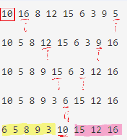
Lets first look at the partition function dry run, using the following example of array.

1. First, as it enters the first loop, 10 is set as pivot and i and j are initialized as shown,
2. Now, i increases till it finds a number greater than 10, and j decreases till it finds an element less than 10.
3. the elements are swapped and the loop continues further, next we find elements 15 and 3 similarly, they swap.
4. Now both the variables are at 6 hence the condition i < j will return false, and the loop exits and we swap the pivot with 6, and we have successfully placed 10.
5. Now we have 2 smaller arrays, shown in yellow and pink, hence the position of 10 is returned from this function.

Quick Sort recursion tree: Example

The above-discussed algorithm was for finding the partition/pivot location of the first node, next the recursion calls twice but for smaller arrays which further trickles downward as shown, Hence this algorithm is also known as divide and rule approach to sorting, another such example is merge sort algorithm

As it can be seen that the program runs multiple loops simultaneously, and can effectively reduce the time complexity if the partition is towards the center, hence we have 2 types of time complexity which will be discussed next.

Time complexity for quicksort algorithm:

Best-case Scenario:

As discussed above if the partition is towards the middle, we get the following equation for solving the time complexity of the program for quicksort algorithm.

T(n) = 2T(n/2) + theta(n)

Which has the solution O(nLogn) which is respectable but not the quickest(more on that later). Next we take a look at the worst case

Worst-case Scenario:

For the worst case, we will have the case where the array is already sorted so the pivot is always the first or last element the equation for this case looks as follows

T(n) = T(n-1) + theta(n)

For this case the solution is O(n2) so we get the worst case time as square of the size of array.

Quick Sort isn’t quickest?

As discussed above, on the contrary to the name, it isn’t the most efficient way to sort an array, for that, you can refer to the merge sort algorithm.